Statistics Complete Notes Chapter Wise Introduction Presentation of Data

These statistics notes chapter wise are original study and revision notes, written in simple language for first-year students who want to understand the ideas first and then practise answering questions. This is not official textbook material, not a board paper, and not leaked material. It does not guarantee any question or mark. Worked numbers in this guide are illustrative examples only, so you can follow the method and then try similar numbers on your own.

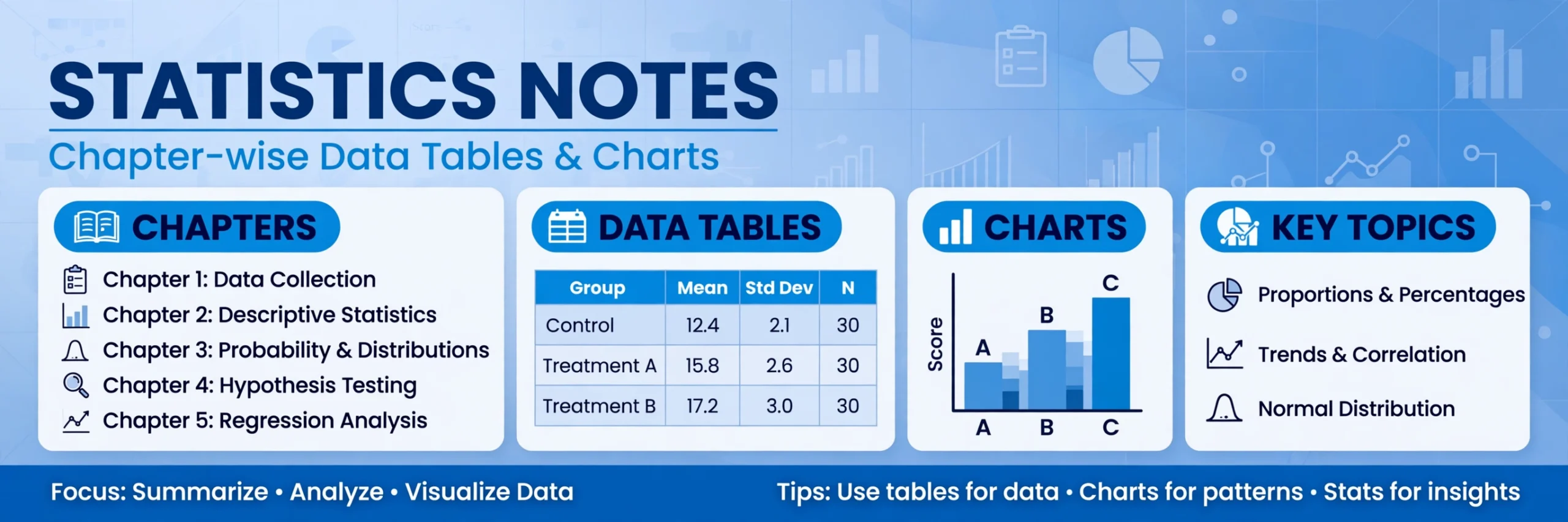
Download the Statistics Notes Chapter Wise PDF

Download Statistics Complete Notes Chapter Wise PDF (Full Question Answers) — use the PDF for offline revision after you have read the explanations below. Each chapter in this post gives an explanation, important points, short questions with full answers, long questions with full answers, and multiple-choice questions with an answer key.

How to Use These Notes

Read one chapter at a time. First learn the meaning in your own words, then look at the worked example, then cover the answers and try the short questions yourself. Only after that, check the answer key for the MCQs. If you are collecting first-year material, also see the 1st Year FBISE All Subjects post and the 1st Year hub for other subjects.

What Is Covered in This Guide

• Chapter 1: Introduction — history, meanings, descriptive and inferential statistics, characteristics, limitations, functions and importance, collection of data, primary and secondary data, variable and constant, accuracy, errors, significant digits, scientific notation, rounding and summation.
• Chapter 2: Presentation of Data — classification, tabulation, frequency distribution, class limits and class boundaries, and charts.
• Chapter 3: Measures of Central Tendency — mean, median and mode.
• Chapter 4: Measures of Dispersion — range, variance and standard deviation.
• Chapter 5: Probability Basics — sample space, event, the 0 to 1 scale, and complement.
• Chapter 6: Index Numbers and Sampling — index numbers with base year equal to 100, and random sampling.

Chapter 1: Introduction

Explanation

Statistics is the study of collecting, organising, presenting, analysing and interpreting numerical information so that sensible decisions can be made. In its early history, statistics was mainly used by states to count people, land and revenue. Later it grew into a general method for studying business, health, education, agriculture and everyday problems where information varies from person to person or place to place. Descriptive statistics describes what is seen in a set of data, for example by giving an average or a table. Inferential statistics goes further: it uses a sample to draw careful conclusions about a larger population, while accepting that some uncertainty remains.

A good statistical study has clear characteristics. It works with facts that can be counted or measured, it deals with groups rather than single isolated cases, and its results should be comparable and open to checking. Its functions are to simplify complex data, compare groups, find relationships, test ideas and help planning. Its importance is practical: a school can compare classes, a shop can judge sales, and a health worker can see whether a problem is growing. Still, statistics has limitations. It cannot study quality alone, such as honesty or kindness, unless those ideas are given a clear measurable form. Results depend on the quality of the data, and a careless conclusion can mislead even when the arithmetic is correct.

Data must be collected carefully. Primary data are collected for the first time, directly for the study in hand, for example by interview, questionnaire or observation. Secondary data were already collected by someone else for another purpose, for example in a published report or official record. Primary data are usually more closely matched to the question but cost more time and effort. Secondary data are quicker and cheaper but may be old, incomplete or defined differently. A variable is a quantity or quality that changes, such as height, marks or income. A constant stays the same in the study, such as the number of days in a particular week used for comparison.

Accuracy means closeness to the true value. Errors can come from a faulty instrument, a biased sample, a wrong question, careless recording or a mistake in calculation. Significant digits show how precise a measurement is: for example, 4.20 has three significant digits, and the final zero matters because it shows the measurement was recorded to two decimal places. In scientific notation a number is written as a value between 1 and 10 multiplied by a power of 10, so 0.00045 becomes 4.5 x 10 to the power -4. Rounding replaces a number by a nearby simpler value: 3.476 rounded to two decimal places is 3.48, because the third decimal, 6, is 5 or more. Summation is shown by the symbol sigma, and the sum of 2, 5 and 7 is written as sigma x = 14.

Important Points: Chapter 1

• Statistics studies numerical facts about groups, not one person alone.
• Descriptive statistics describes data; inferential statistics draws conclusions about a population from a sample.
• Primary data are new and purpose-built; secondary data already exist.
• A variable changes; a constant does not change in the study.
• Always state the unit, check the source, and treat rounded or sampled results as approximate, not exact truth.

Chapter 1: Short Questions With Answers

1. What is statistics? Answer: Statistics is the science of collecting, organising, presenting, analysing and interpreting numerical data. Its purpose is to turn scattered figures into clear information that can support a decision, rather than leaving the reader to guess from raw numbers.
2. What is the difference between descriptive and inferential statistics? Answer: Descriptive statistics summarises the data actually collected, for example through a table, chart or average. Inferential statistics uses a sample to make a reasoned conclusion about a wider population, and that conclusion always carries some uncertainty.
3. What is the difference between primary and secondary data? Answer: Primary data are collected afresh for the current study, such as by a survey the researcher carries out. Secondary data already exist and were collected by someone else, such as figures in an official report. Primary data fit the question better, while secondary data save time but need checking for age and definitions.
4. Define variable and constant with one example each. Answer: A variable changes from case to case, for example the marks of students in a class. A constant does not change during the study, for example if every student is tested on the same 100-mark paper, the total marks of 100 is constant for that study.
5. Round 3.476 to two decimal places and explain the rule. Answer: 3.48. Look at the third decimal place, which is 6. Because it is 5 or more, the second decimal place, 7, is increased by one to 8, and the remaining digits are dropped.

Chapter 1: Long Questions With Answers

1. Explain the functions and importance of statistics, and state its main limitations. Answer: Statistics simplifies large sets of figures, makes comparison possible, helps to find relationships, supports forecasting and planning, and gives a basis for testing claims. It is important because governments, schools, hospitals and businesses all make decisions about groups, and they need reliable summaries rather than impressions. Its limitations must also be remembered: it studies numbers and groups, so a quality such as kindness cannot be measured directly; a result is only as good as the data and method behind it; and statistics can be misused if figures are chosen selectively or shown without context. A good answer therefore uses statistics as evidence, not as proof by itself.
2. Explain collection of data, accuracy, significant digits and scientific notation, with examples. Answer: Data may be collected directly for the study, giving primary data, or taken from existing sources, giving secondary data. The choice depends on time, cost, accuracy needed and whether suitable data already exist. Accuracy means closeness to the true value, and errors may come from sampling, questioning, recording or calculation. Significant digits show precision: 4.20 is more precise than 4.2 because it is recorded to two decimal places. Scientific notation writes very large or small numbers clearly, for example 0.00045 = 4.5 x 10 to the power -4, and 45,000 = 4.5 x 10 to the power 4. Together these ideas help a student record, report and judge numbers honestly.

Chapter 1: MCQs and Answer Key

1. Statistics mainly deals with: (a) single opinions (b) numerical facts about groups (c) personal feelings only (d) unrecorded stories — Answer: (b)
2. Descriptive statistics is used to: (a) predict without data (b) summarise collected data (c) ignore variation (d) replace sampling — Answer: (b)
3. Data collected for the first time for a study are called: (a) secondary data (b) primary data (c) estimated data (d) historical data — Answer: (b)
4. Which of the following is a variable? (a) 100 marks for every paper (b) height of students (c) 7 days in a week (d) 12 months in a year — Answer: (b)
5. 45,000 in scientific notation is: (a) 4.5 x 10 to the power 3 (b) 4.5 x 10 to the power 4 (c) 45 x 10 to the power 4 (d) 0.45 x 10 to the power 5 — Answer: (b)

Chapter 2: Presentation of Data

Explanation

Raw data are hard to read, so they are first classified and then presented. Classification means grouping data by a common feature, for example by class, by marks, by place or by time. A table then arranges the grouped data in rows and columns with a clear title, column headings, units and a total where useful. Tabulation makes comparison easy and prepares the data for charts and calculations. A good table is simple, complete and self-explanatory: a reader should understand it without searching the whole text.

A frequency distribution groups values into classes and shows how many observations fall in each class. For example, marks from 0 to 100 might be grouped as 0-9, 10-19, 20-29 and so on, with the frequency showing how many students are in each group. Class limits are the stated lower and upper values of a class, such as 10 and 19 in the class 10-19. Class boundaries are different: they are the true dividing points between classes. If classes are 10-19 and 20-29, the boundary between them is 19.5, because the gap of 1 is split equally, 0.5 on each side. The width of a class is the difference between two successive boundaries, here 10. The midpoint is the average of the lower and upper boundaries, for 10-19 it is 14.5.

Charts turn a table into a picture. A bar chart uses bars to compare categories, a histogram uses touching bars for continuous grouped data, a frequency polygon joins the midpoints of histogram bars, and a pie chart shows parts of a whole as slices. A bar chart is best when categories are separate, while a histogram is best when data are grouped in a continuous scale. Always label the axes, give the chart a title, use the same scale throughout, and do not stretch an axis in a way that exaggerates a small difference.

Important Points: Chapter 2

• Classification groups data; tabulation arranges it in rows and columns.
• A frequency distribution shows classes and how many values are in each class.
• Class limits are the stated values; class boundaries are the true dividing points.
• For classes 10-19 and 20-29, the boundary is 19.5 and the class width is 10.
• Choose the chart to match the data: bars for categories, histogram for continuous grouped data, pie chart for parts of a whole.

Chapter 2: Short Questions With Answers

1. What is classification? Answer: Classification is grouping data by a shared feature, such as age group, subject or region. It turns a long, mixed list into orderly groups that can be compared and summarised.
2. What is tabulation? Answer: Tabulation is presenting classified data in a table with rows, columns, a title and headings. A good table is clear, complete and can be understood on its own, without extra explanation.
3. What is a frequency distribution? Answer: A frequency distribution divides data into classes and records how many observations fall in each class. For example, if 8 students score 10-19 and 12 score 20-29, those numbers, 8 and 12, are the frequencies of those classes.
4. What is the difference between class limits and class boundaries? Answer: Class limits are the values written for a class, such as 10 and 19 for the class 10-19. Class boundaries are the real dividing points between classes. Between 10-19 and 20-29 the boundary is 19.5, because the gap between 19 and 20 is split in half.
5. When is a histogram used instead of a bar chart? Answer: A histogram is used for continuous grouped data, with bars that touch each other to show an unbroken scale. A bar chart is used for separate categories, with gaps between bars, because the categories do not form a continuous scale.

Chapter 2: Long Questions With Answers

1. Explain frequency distribution, class width, midpoint and class boundaries with an illustrative example. Answer: Suppose marks are grouped as 0-9, 10-19, 20-29 and 30-39. The frequencies might be 4, 9, 11 and 6, meaning 4 students in the first class, 9 in the second, and so on, with a total of 30 students. The class width is 10, found from the distance between successive boundaries. For the class 10-19 the boundaries are 9.5 and 19.5, and the midpoint is (9.5 + 19.5) divided by 2, which is 14.5. Boundaries matter because they remove the gap between written classes and allow a histogram to be drawn on a continuous scale. A student who confuses limits with boundaries will get the midpoint and the chart wrong, so both ideas should be stated in the answer.
2. Explain how to choose a chart and what makes a chart honest. Answer: First ask what the data show. Use a bar chart to compare separate categories, a histogram for grouped continuous data, a frequency polygon to show the shape of a distribution, and a pie chart only when the parts make up one whole. An honest chart has a clear title, labelled axes, a single consistent scale, and no broken or stretched axis that exaggerates a small difference. It should also show the source or the total where that helps the reader judge the picture. A chart that looks impressive but hides the scale or the total is not a good presentation, even if it is colourful.

Chapter 2: MCQs and Answer Key

1. Grouping data by a common feature is called: (a) tabulation (b) classification (c) estimation (d) sampling — Answer: (b)
2. In the class 10-19, the upper class limit is: (a) 9.5 (b) 10 (c) 19 (d) 19.5 — Answer: (c)
3. Between classes 10-19 and 20-29, the class boundary is: (a) 19 (b) 19.5 (c) 20 (d) 20.5 — Answer: (b)
4. A histogram is used for: (a) separate categories (b) parts of a whole (c) continuous grouped data (d) two variables only — Answer: (c)
5. A pie chart is most suitable when: (a) data are in classes (b) parts make up a whole (c) values are negative (d) no total exists — Answer: (b)

Chapter 3: Measures of Central Tendency

Explanation

A measure of central tendency gives one typical value for a set of data. The mean is the arithmetic average: add all values and divide by how many there are. For 4, 6 and 8, the mean is (4 + 6 + 8) divided by 3, which is 6. The median is the middle value when data are arranged in order. For 3, 7, 9, 12 and 20, the median is 9. If there are two middle values, take their average. The mode is the value that occurs most often; a set can have one mode, more than one mode, or no mode if every value occurs once.

Each measure suits a different situation. The mean uses every value, so it is useful for further calculation, but one very large or very small value can pull it away from the typical value. The median is not pulled in the same way, so it is useful when data are skewed or contain an extreme value. The mode is useful for categories, such as the most common shoe size, where an average may not make sense. A good answer names the measure, shows the working, and says why that measure was chosen.

Important Points: Chapter 3

• Mean = sum of values divided by number of values.
• Median = middle value after arranging data in order.
• Mode = most frequent value.
• The mean is sensitive to extreme values; the median is more resistant.
• For grouped data, the class with the highest frequency is the modal class.

Chapter 3: Short Questions With Answers

1. Find the mean of 4, 6 and 8. Answer: Add the values, 4 + 6 + 8 = 18, and divide by 3, giving 6.
2. Find the median of 3, 7, 9, 12 and 20. Answer: The values are already in order and there are five of them, so the middle, third, value is 9.
3. Find the mode of 2, 5, 5, 7 and 9. Answer: 5, because it occurs twice while every other value occurs once.
4. Why can the mean be misleading? Answer: Because the mean uses every value, a single very large or very small value can pull it away from most of the data, so it may not represent a typical case.
5. When is the mode the best choice? Answer: When the data are categories or when the most common case is needed, such as the most popular size, because mean and median do not apply in the same way to labels.

Chapter 3: Long Questions With Answers

1. Find the mean, median and mode of 5, 8, 8, 12, 15 and 20, and comment on the results. Answer: The mean is (5 + 8 + 8 + 12 + 15 + 20) divided by 6, which is 68 divided by 6, about 11.33. The values are in order, and with six values the median is the average of the third and fourth values, (8 + 12) divided by 2, which is 10. The mode is 8, the only repeated value. The mean is higher than the median because the larger values, 15 and 20, pull it up, while the median stays near the centre. This shows why comparing two measures can reveal the shape of the data.
2. Explain the uses and limitations of mean, median and mode. Answer: The mean is useful because it uses all values and can be used in further work, but it is affected by extreme values and cannot be used for simple categories. The median is useful for skewed data and is easy to understand as the middle value, but it ignores how far other values are from the centre. The mode is simple and works for categories, but it may not exist, there may be more than one mode, and it ignores most values. A careful student therefore chooses the measure that matches the data and the question, and states the reason in the answer.

Chapter 3: MCQs and Answer Key

1. The mean of 4, 6 and 8 is: (a) 5 (b) 6 (c) 7 (d) 18 — Answer: (b)
2. The median of 3, 7, 9, 12 and 20 is: (a) 7 (b) 9 (c) 12 (d) 10 — Answer: (b)
3. The mode of 2, 5, 5, 7 and 9 is: (a) 2 (b) 7 (c) 5 (d) 9 — Answer: (c)
4. Which measure is most affected by an extreme value? (a) mode (b) median (c) mean (d) range — Answer: (c)
5. Which measure is best for the most common category? (a) mean (b) median (c) mode (d) variance — Answer: (c)

Chapter 4: Measures of Dispersion

Explanation

An average alone does not tell the whole story, because two groups can have the same mean but very different spread. Measures of dispersion describe that spread. The range is the simplest: it is the largest value minus the smallest value. For 4, 7, 9 and 12, the range is 12 minus 4, which is 8. It is quick to find, but it uses only two values, so one extreme value can change it a lot.

Variance and standard deviation use every value. First find the mean, then find how far each value is from the mean, square each distance, and average those squared distances. That average is the variance. The standard deviation is the square root of the variance, and it brings the result back to the original units, such as marks or centimetres. For the illustrative values 2, 4, 4, 4, 5, 5, 7 and 9, the mean is 5, the squared distances are 9, 1, 1, 1, 0, 0, 4 and 16, their sum is 32, the variance is 32 divided by 8, which is 4, and the standard deviation is the square root of 4, which is 2. A small standard deviation means values cluster near the mean; a large one means they are widely spread.

Important Points: Chapter 4

• Range = maximum value minus minimum value.
• Variance is the average of the squared distances from the mean.
• Standard deviation is the square root of the variance.
• Standard deviation is in the same units as the data; variance is in squared units.
• Two sets with the same mean can have very different dispersion.

Chapter 4: Short Questions With Answers

1. Find the range of 4, 7, 9 and 12. Answer: 12 minus 4 = 8.
2. What is variance? Answer: Variance is the average of the squared differences between each value and the mean. Squaring removes negative signs, so distances above and below the mean do not cancel each other.
3. What is standard deviation? Answer: Standard deviation is the square root of the variance. It measures typical distance from the mean, in the same units as the original data.
4. Why is the range a weak measure? Answer: Because it uses only the smallest and largest values, so it ignores all other values and is easily changed by one extreme value.
5. What does a small standard deviation mean? Answer: It means most values lie close to the mean, so the group is fairly consistent. A large standard deviation means the values are widely spread.

Chapter 4: Long Questions With Answers

1. Find the variance and standard deviation of 2, 4, 4, 4, 5, 5, 7 and 9. Answer: First find the mean: the sum is 40, divided by 8, giving 5. The distances from 5 are -3, -1, -1, -1, 0, 0, 2 and 4. Squaring them gives 9, 1, 1, 1, 0, 0, 4 and 16, whose sum is 32. The variance is 32 divided by 8, which is 4. The standard deviation is the square root of 4, which is 2. The answer should show each step, because a missing step makes it hard to find a small arithmetic error.
2. Compare range, variance and standard deviation, and explain why dispersion matters. Answer: Range is the quickest measure but the least reliable, because it depends on only two values. Variance uses all values and measures spread precisely, but its units are squared, which is hard to interpret. Standard deviation solves that problem by taking the square root, giving a spread in the original units. Dispersion matters because averages hide differences: two classes can have the same mean mark, yet one may be consistent while the other has very high and very low marks. A decision based only on the mean could therefore be misleading.

Chapter 4: MCQs and Answer Key

1. The range of 4, 7, 9 and 12 is: (a) 4 (b) 8 (c) 9 (d) 12 — Answer: (b)
2. Variance is: (a) sum of distances (b) average of squared distances from the mean (c) largest minus smallest (d) square root of the mean — Answer: (b)
3. Standard deviation is: (a) variance squared (b) square root of variance (c) mean minus mode (d) range divided by 2 — Answer: (b)
4. If variance is 4, standard deviation is: (a) 16 (b) 8 (c) 4 (d) 2 — Answer: (d)
5. A large standard deviation shows: (a) values close to the mean (b) values widely spread (c) no variation (d) equal values — Answer: (b)

Chapter 5: Probability Basics

Explanation

Probability measures how likely an outcome is, on a scale from 0 to 1. A probability of 0 means the outcome cannot happen, a probability of 1 means it is certain, and a probability of 0.5 means it is equally likely to happen or not. An experiment is an action with an uncertain result, such as tossing a coin. The sample space is the set of all possible outcomes of that experiment. For one coin toss, the sample space is heads and tails. An event is a set of outcomes of interest, such as getting heads.

For equally likely outcomes, the probability of an event is the number of favourable outcomes divided by the total number of possible outcomes. For one fair die, the probability of getting a 4 is 1 divided by 6, because there is one favourable outcome out of six. The complement of an event is everything in the sample space that is not in the event. If the probability of an event is P, then the probability of its complement is 1 minus P. So if the probability of rain is 0.3, the probability of no rain is 0.7. This rule is useful when the complement is easier to count than the event itself.

Important Points: Chapter 5

• Probability lies between 0 and 1, inclusive.
• Sample space = all possible outcomes; event = outcomes of interest.
• For equally likely outcomes, probability = favourable outcomes divided by total outcomes.
• Complement rule: P(not A) = 1 minus P(A).
• A probability is never negative and never greater than 1.

Chapter 5: Short Questions With Answers

1. What is a sample space? Answer: The sample space is the set of all possible outcomes of an experiment. For tossing one coin it is heads and tails; for rolling one die it is 1, 2, 3, 4, 5 and 6.
2. What is an event? Answer: An event is a collection of outcomes from the sample space that we are interested in, such as getting an even number on a die, which is the outcomes 2, 4 and 6.
3. What do probabilities 0 and 1 mean? Answer: 0 means impossible, so the outcome cannot happen, and 1 means certain, so the outcome must happen. Values between 0 and 1 show increasing likelihood.
4. Find the probability of getting a 4 on a fair die. Answer: There is one favourable outcome, 4, out of six equally likely outcomes, so the probability is 1 divided by 6, about 0.167.
5. If P(A) = 0.3, what is P(not A)? Answer: By the complement rule, P(not A) = 1 minus 0.3 = 0.7.

Chapter 5: Long Questions With Answers

1. Explain sample space, event and probability using a die, and find the probability of an even number. Answer: Rolling a die is an experiment because the result is uncertain. Its sample space is 1, 2, 3, 4, 5 and 6. The event of getting an even number is the set 2, 4 and 6. There are three favourable outcomes out of six possible outcomes, so the probability is 3 divided by 6, which is 0.5. This also shows the method in general: list the sample space, identify the event, count both, and divide, but only when the outcomes are equally likely.
2. Explain the 0 to 1 probability scale and the complement rule, with an example. Answer: Probability cannot be less than 0 or greater than 1, because an event cannot happen less than never or more than always. A value near 0 is unlikely, 0.5 is equally likely, and a value near 1 is very likely. The complement of an event contains all outcomes not in that event, and together an event and its complement cover the whole sample space, so their probabilities add to 1. For example, if the probability of picking a red ball from a bag is 0.4, the probability of not picking a red ball is 1 minus 0.4, which is 0.6. Checking that a calculated probability lies between 0 and 1 is a useful final step.

Chapter 5: MCQs and Answer Key

1. Probability of an impossible event is: (a) 1 (b) 0.5 (c) 0 (d) -1 — Answer: (c)
2. Sample space for one coin toss is: (a) heads only (b) tails only (c) heads and tails (d) two heads — Answer: (c)
3. Probability of getting a 4 on a fair die is: (a) 1/2 (b) 1/3 (c) 1/6 (d) 4/6 — Answer: (c)
4. If P(A) = 0.3, P(not A) is: (a) 0.3 (b) 0.7 (c) 1.3 (d) 0 — Answer: (b)
5. Probability of a certain event is: (a) 0 (b) 0.5 (c) 1 (d) 2 — Answer: (c)

Chapter 6: Index Numbers and Sampling

Explanation

An index number compares a value in a later period with the same value in a base period, using one simple number. The base year is given the value 100, and other years are expressed against it. The formula is: index number = (value in the current year divided by value in the base year) multiplied by 100. For example, if a price is 50 in the base year and 60 in the current year, the index is (60 divided by 50) multiplied by 100, which is 120. That means the price has risen by 20 percent from the base year. If the index were 90, the value would have fallen by 10 percent from the base year.

Sampling is the study of part of a population to learn about the whole. A population is all the cases of interest, while a sample is a smaller group chosen from it. In random sampling, every member of the population has an equal chance of being chosen, which reduces the risk of a biased sample. A simple way to do this is to list the population, assign numbers, and choose numbers by a lottery or a random-number method. Random sampling does not remove all error, but it gives a fair basis for generalising, provided the sample is large enough and the method is followed honestly.

Important Points: Chapter 6

• Base year index = 100 by definition.
• Index = (current value / base value) x 100.
• Index 120 means a 20 percent rise from the base year; index 90 means a 10 percent fall.
• Population = all cases; sample = part chosen for study.
• In random sampling every member has an equal chance of selection.

Chapter 6: Short Questions With Answers

1. What is an index number? Answer: An index number is a single number that shows how a value, such as a price, has changed compared with a base period. It makes comparison easy even when the original values are large or in different units.
2. Why is the base year set to 100? Answer: Setting the base year to 100 gives a fixed starting point. Later values can then be read at a glance: above 100 means a rise, below 100 means a fall, and the distance from 100 shows the percentage change.
3. A price rises from 50 to 60. Find the index number. Answer: (60 divided by 50) multiplied by 100 = 120, so the price has risen by 20 percent from the base year.
4. What is the difference between population and sample? Answer: The population is the whole group of interest, while a sample is a smaller part of that group actually studied. Conclusions from a sample are used to learn about the population.
5. What is random sampling? Answer: Random sampling is a method in which every member of the population has an equal chance of being selected. It reduces personal bias in choosing who is included.

Chapter 6: Long Questions With Answers

1. Explain index numbers with a worked example, and state what values above and below 100 mean. Answer: An index number compares a current value with a base-year value. Take a base-year price of 80 and a current price of 100. The index is (100 divided by 80) multiplied by 100, which is 125, meaning a 25 percent rise. If instead the current price were 72, the index would be (72 divided by 80) multiplied by 100, which is 90, meaning a 10 percent fall. Index numbers are therefore useful for tracking prices, production or wages over time without being distracted by the size of the original figures, but the choice of base year matters, so it should be a normal, representative year.
2. Explain random sampling, its steps, and why it is preferred to a biased choice. Answer: Random sampling begins by defining the population clearly, listing its members, and giving each member an equal chance of selection, for example by drawing lots or using random numbers. The chosen sample is then studied, and results are generalised with care. It is preferred to a biased choice because the researcher cannot, even unconsciously, pick only convenient or favourable cases. Random sampling does not guarantee a perfect sample, especially if the sample is very small, but it removes selection bias and gives a defensible basis for conclusions about the population.

Chapter 6: MCQs and Answer Key

1. Base year index number is: (a) 0 (b) 10 (c) 100 (d) 1000 — Answer: (c)
2. If price rises from 50 to 60, the index is: (a) 110 (b) 120 (c) 150 (d) 60 — Answer: (b)
3. An index of 90 means: (a) 90 percent rise (b) 10 percent fall (c) no change (d) 90 percent fall — Answer: (b)
4. A sample is: (a) the whole population (b) a part of the population studied (c) a census (d) a single value — Answer: (b)
5. In random sampling, every member has: (a) no chance (b) an equal chance (c) a chosen chance (d) a different fixed chance — Answer: (b)

Revision Checklist

• Can you explain descriptive and inferential statistics, primary and secondary data, variable and constant, rounding and scientific notation?
• Can you build a frequency distribution, find class boundaries and midpoints, and choose a suitable chart?
• Can you find mean, median and mode, and say which measure fits the data?
• Can you find range, variance and standard deviation, and explain what spread means?
• Can you list a sample space, find a probability, and use the complement rule?
• Can you calculate an index number from a base year of 100 and explain random sampling?
• Have you tried all short and long questions without looking, and checked the MCQ answer keys?
• Have you downloaded the PDF for offline revision from the link at the top of this post?

For more first-year material, return to the 1st Year FBISE All Subjects post and the 1st Year hub. These are original study and revision notes only, not official textbook notes, not board papers, not leaked material, and not a guarantee of any question or mark.